Blog Posts: Feature Selection via Gain Penalization in Random Forests

Bruna Wundervald

doi:10.1109/ACCESS.2020.3032095

Introduction

Decision trees ensembles are a very popular type of machine learning algorithm, which is mostly due to their adaptive nature, high prediction power and, in some sense, interpretability. Random Forests are one form of such ensembles, and they consist of growing many trees in re-samples of the data, and averaging their results at end, creating a bagged ensemble described (Breiman 1996) by

\[\begin{equation} \hat f(\mathbf{x}) = \sum_{n = 1}^{N_{tree}} \frac{1}{N_{tree}} \hat f_n(\mathbf{x}), \end{equation}\]

where $\hat f_n$ corresponds to the $n$-th tree. However, even though we can name many very good qualities of the Random Forests, we also know that they don’t do feature selection very well. However, Random Forests usually use all or most of the features that are feed to them, and they struggle a lot to detect highly correlated features (Louppe 2014), that ideally shouldn’t be used in an algorithm more than once. In a situation where predictions are hard or expensive to obtain (e.g. genetic related data such as SNPs, peptides or proteins), this becomes a relevant issue that needs to be addressed if we realistically want to use RFs for such prediction tasks.

In this post, I will give a general overview of feature selection in Random Forests using gain penalization. The R code is provided along with the explanation, and I’ll often be referring to my own paper on the subject (Wundervald, Parnell, and Domijan 2020). A few auxiliary functions are used throughout the code, and they can be found here.

What is Gain Penalization?

The idea of doing feature selection via gain penalization was first introduced in (Deng and Runger 2012), and it is basically a gain weighting method, done during the greedy procedure step of a tree estimation. In other words, when determining the next child node to be added to a decision tree, the gain (or the error reduction) of each feature is multiplied by a penalization parameter. With this, a new split will only be made if, after the penalization, the gain of adding this node is still higher than having no new child node in the tree. This new penalized gain is written as

\[\begin{equation} \text{Gain}_{R}(\mathbf{X}_{i}, t) = \begin{cases} \lambda \Delta(i, t), \thinspace i \notin \mathbb{U} \text{ and} \\ \Delta(i, t), \thinspace i \in \mathbb{U}, \end{cases} \label{eq:grrf} \end{equation}\]

where $\mathbb{U}$ is the set of indices of the features previously used in the tree, $\mathbf{X}_{i}$ is the candidate feature, $t$ is the candidate splitting point and $\lambda \in (0, 1]$.

In our paper (Wundervald, Parnell, and Domijan 2020), we proposed a generalization to the way the penalization coefficients are calculated, such that we can have full control over it. Our $\lambda_i$ is written as

\[\begin{equation} \lambda_i = (1 - \gamma) \lambda_0 + \gamma g(\mathbf{x}_i), \label{eq:generalization} \end{equation}\]

where $\lambda_0 \in [0, 1)$ is interpreted as the baseline regularization, $g(\mathbf{x}_i)$ is a function of the $i$-th feature, and $\gamma \in [0, 1)$ is their mixture parameter, with $\lambda_i \in [0, 1)$. The idea behind this composition is creating a local-global form of penalization, since the equation mixes how much all features are jointly (globally) penalized and how much it is due to a local $g(\mathbf{x}_i)$, which is manually defined. This $g(\mathbf{x}_i)$, by its turn, should represent relevant information about the features, based on some characteristic of interest (correlation to the target, for example). This formulation also has inspiration on the use of priors made in Bayesian methods, since we introduce “prior knowledge” regarding the importance of each feature into the model (likewise, the data will tell us how strong our assumptions about the penalization are, since even if we try to penalize a truly important feature, its gain will be high enough to overcome the penalization and the feature will get selected by the algorithm).

In this blog post, I’ll use two different types of $g(\mathbf{x}_i)$:

The Mutual Information between each feature and the target variable $y$ (normalized to be between 0 and 1)
The variable importance values obtained from a previously run standard Random Forest, which is what I call a Boosted $g(\mathbf{x}_i)$
(also normalized to be between 0 and 1)

For more details on those functions and other options, please see the paper (Wundervald, Parnell, and Domijan 2020).

The full feature selection procedure

In general, the penalized random forest model is not the one that will be used for the final predictions. Instead, I prefer to use the method described before as a tool to first select the best features possible, and then have a final random forest that uses such features. This full feature selection procedure happens in 3 main steps:

We run a bunch of penalized random forests models with different hyperparameters and record their accuracies and final set of features
For each training dataset, select the top-n (for this post we use n = 3) fitted models in terms of the accuracies, and run a “new” random forest for each of the feature sets used by them. This is done using all of the training sets so we can evaluate how these features perform in slightly different scenarios
Finally, get the top-m set of models (here m = 30) from these new ones, check which features were the most used between them and run a final random forest model with this feature set. In this post I select only the 15 most used features from the top 30 models, but both numbers can be changed depending on the situation

All this is to make sure that the features used in the final model are, indeed, very good. This might sound a bit exhaustive but to me it pays off knowing that out of a few thousand variables, I’ll manage to select only a few and still have a powerful and generalizable model.

Things to have in mind when running the penalized RF

You can add an “extra penalization” when the new variable is to be picked at a deep node in a tree (for details please see the paper)
The mtry hyperparameter requires attention (and even proper tuning), since it is known that to affect the prediction power of random forests and, is our case, the penalized random forests
Ideally, the $\gamma$, $\lambda_0$ and mtry hyperparameters should be tuned, or set based on the experience of the person running the algorithms, but for the time being we’ll be using a few predefined values (kind of like grid search)

Implementation

Let us consider the gravier dataset (Gravier et al. 2010), for which the goal is to predict whether 168 breast cancer patients had a diagnosis labelled “poor” (~66%) or “good” (~33%), based on a a set of 2905 predictors. In this first part of the code, we’ll just load the data and create our 5-fold cross validation object, which will be used to create 5 different train and test sets. As of usual, there will be lots of tidyverse and tidymodels functions throughout my code:


library(tidyverse)
library(tidymodels)
library(infotheo) # For the mutual information function
set.seed(2021)

# Loading data and creating a 5-fold CV object
data('gravier', package = 'datamicroarray')

gravier <- data.frame(class = gravier$y, gravier$x)
folds <- rsample::vfold_cv(gravier, v = 5) %>% 
  dplyr::mutate(train =  map(splits, training),
                test  = map(splits, testing))

With this done, we can start the actual modelling steps of the code. I will be using a few of auxiliary functions, which are given here, but the two following functions are explicitly shown in this post because they’re very important. The modelling() function will be used to run the random forests algorithms, and it’s written in a way that I can change the mtry hyperparameter, the penalization coefficients. At this point we’ll be feeding all the 2905 features, and letting the gain penalization perform the feature selection for us. The second function shown below is penalization(), which implements the calculation of two different types of penalization: one that takes $g(\mathbf{x}_i)$ to be the normalized mutual information between the target and each feature, and one that I call a “Boosted” $g(\mathbf{x}_i)$, because it depends on the normalized importance values of a previously calculated random forest (for more details, see Wundervald, Parnell, and Domijan (2020)).


# A function that run the penalized random forests models 
modelling <- function(train, reg_factor = 1, mtry = 1){
  rf_mod <- 
    rand_forest(trees = 500, mtry = (mtry * ncol(train)) - 1) %>% 
    set_engine("ranger", importance = "impurity", 
               regularization.factor = reg_factor) %>% 
    set_mode("classification") %>% 
    parsnip::fit(class ~ ., data = train)
  return(rf_mod)
}
# A function that receives the mixing parameters
# and calculates lambda_i with the chose g(x_i)
penalization <- function(gamma, lambda_0, data = NULL, imps = NULL, type = "rf"){
  if(type == "rf"){
    # Calculating the normalized importance values 
    imps <- imps/max(imps)
    imp_mixing <- (1 - gamma) * lambda_0 + imps * gamma 
    return(imp_mixing)
  } else if(type == "MI"){
    mi <- function(data, var) mutinformation(c(data$class), data %>% pull(var))
    
    # Calculating the normalized mutual information values
    disc_data  <- infotheo::discretize(data) 
    disc_data$class <- as.factor(data$class)
    names_data <- names(data)[-1]
    mi_vars <- names_data  %>% map_dbl(~{mi(data = disc_data, var = .x) })
    mi_mixing <- (1 - gamma) * lambda_0 + gamma * (mi_vars/max(mi_vars))
    return(mi_mixing)  
  }
}

The code below creates the combinations of all hypeparameter values used here, for the $\gamma$, $\lambda_0$ and mtry hyperparameters. After that, we calculate the two $g(\mathbf{x}_i)$ for each training set, and their final coefficient penalization values by combining them with $\gamma$ and $\lambda_0$ to create the penalization mixture (as described previously), for each of the 5 training sets.


# Setting all parameters ---
mtry <-  tibble(mtry = c(0.20, 0.45, 0.85))  
gamma_f  <-  c(0.3, 0.5, 0.8)
lambda_0_f <- c(0.35, 0.75)

parameters <- mtry %>% tidyr::crossing(lambda_0_f, gamma_f)
# Adds gamma_f and lambda_0_f and run the functions with them ------
folds_imp <- folds %>% 
  dplyr::mutate(
    # Run the standard random forest model for the 5 folds
    model = purrr::map(train, modelling), 
    importances_std = purrr::map(model, ~{.x$fit$variable.importance}))  %>%
  tidyr::expand_grid(parameters) %>% 
  dplyr::mutate(imp_rf = purrr::pmap(
    list(gamma_f, lambda_0_f, train, importances_std), type = "rf", 
    penalization), 
    imp_mi = purrr::pmap(
      list(gamma_f, lambda_0_f, train, importances_std), type = "MI", penalization))

A quick look at :


# A tibble: 3 x 7
  id    reg_factor     mtry lambda_0_f gamma_f imp_rf      imp_mi     
  <chr> <list>        <dbl>      <dbl>   <dbl> <list>      <list>     
1 Fold1 <dbl [2,905]>   0.2       0.35     0.3 <dbl [2,90… <dbl [2,90…
2 Fold1 <dbl [2,905]>   0.2       0.35     0.5 <dbl [2,90… <dbl [2,90…
3 Fold1 <dbl [2,905]>   0.2       0.35     0.8 <dbl [2,90… <dbl [2,90…

The folds_imp object has 90 rows, since it is the combination of 2 $\times$ 3 $\times$ 3 hyperparameter combinations for each of the 5 training sets, and 2 different $g(\mathbf{x}_i)$. Before running our penalized models, we take a look at the results for the standard random forests models (the model column). Here, the accuracy and accuracy_std columns represent the test accuracy and training accuracy from a non-penalized RF, which was run before to create the penalization coefficients, so now we can use it for comparison:


folds_imp %>% 
  dplyr::group_by(id) %>% 
  dplyr::slice(1) %>% 
  dplyr::ungroup() %>% 
  dplyr::select(id, model, train, test) %>% 
  dplyr::mutate(
    model_importance = purrr::map(model, ~{.x$fit$variable.importance}),
    n_var = purrr::map_dbl(model_importance, n_vars), 
    accuracy_test_std = purrr::map2_dbl(
      .x = model, .y = test, ~{ acc_test(.x, test = .y)}),
    accuracy_std = 1 -purrr::map_dbl(model, ~{ .x$fit$prediction.error})
  ) %>% 
  dplyr::select(id, n_var, accuracy_test_std, accuracy_std)

id	n_var	accuracy_test_std	accuracy_std
Fold1	1206	0.735	0.8481872
Fold2	1380	0.765	0.8235503
Fold3	1379	0.765	0.8246055
Fold4	1377	0.788	0.8260160
Fold5	1198	0.667	0.8548713

The following code runs all the penalized random forests models and calculates their metrics.


run_all_models <-  folds_imp %>%   
  dplyr::select(id, model, train, test,  imp_rf, imp_mi, mtry, lambda_0_f, gamma_f) %>% 
  tidyr::gather(type, importance, -train, -test, -mtry,-id, -model, -lambda_0_f, -gamma_f) %>% 
  dplyr::mutate(fit_penalized_rf = purrr::pmap(list(train, importance, mtry), modelling))

And finally we extract the metrics we’re interested in, from each estimated model: the number of features used, accuracy in the test set, and the accuracy calculated during training:


results <- run_all_models %>% 
  dplyr::mutate(
    model_importance = purrr::map(fit_penalized_rf, ~{.x$fit$variable.importance}),
    n_var = purrr::map_dbl(model_importance, n_vars),
    accuracy = 1 - purrr::map_dbl(fit_penalized_rf, ~{ .x$fit$prediction.error}),
    accuracy_test = purrr::map2_dbl(
      .x = fit_penalized_rf, .y = test, ~{ acc_test(.x, .y)}))

A quick look at the results object:


results %>% 
  dplyr::arrange(id, desc(accuracy_test), desc(accuracy), n_var) %>% 
  dplyr::slice(1:5)

id	mtry	lambda_0_f	gamma_f	type	n_var	accuracy	accuracy_test
Fold1	0.85	0.75	0.5	imp_rf	5	0.8979667	0.824
Fold1	0.20	0.75	0.3	imp_rf	32	0.8786310	0.794
Fold1	0.45	0.75	0.8	imp_rf	12	0.9001406	0.765
Fold1	0.45	0.35	0.3	imp_rf	11	0.8998857	0.765
Fold1	0.45	0.35	0.5	imp_rf	13	0.8995989	0.765

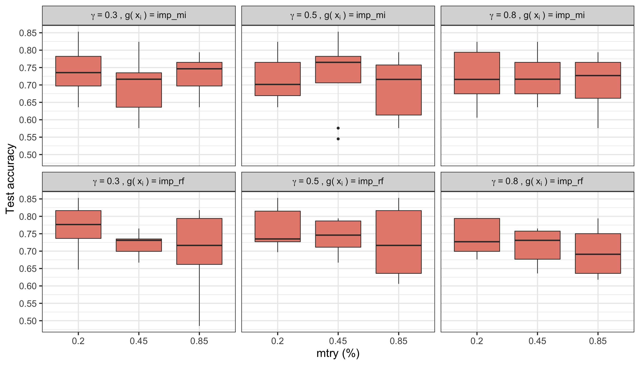
$Figure 1. Test accuracies for each combination of mtry, type of $g(\mathbf{x}_i)$, and $\gamma$.$

Figure 1: Figure 1. Test accuracies for each combination of mtry, type of $g(\mathbf{x}_i)$, and $\gamma$.

$Figure 2. Final number of variables used for each combination of mtry, type of $g(\mathbf{x}_i)$, and $\gamma$$

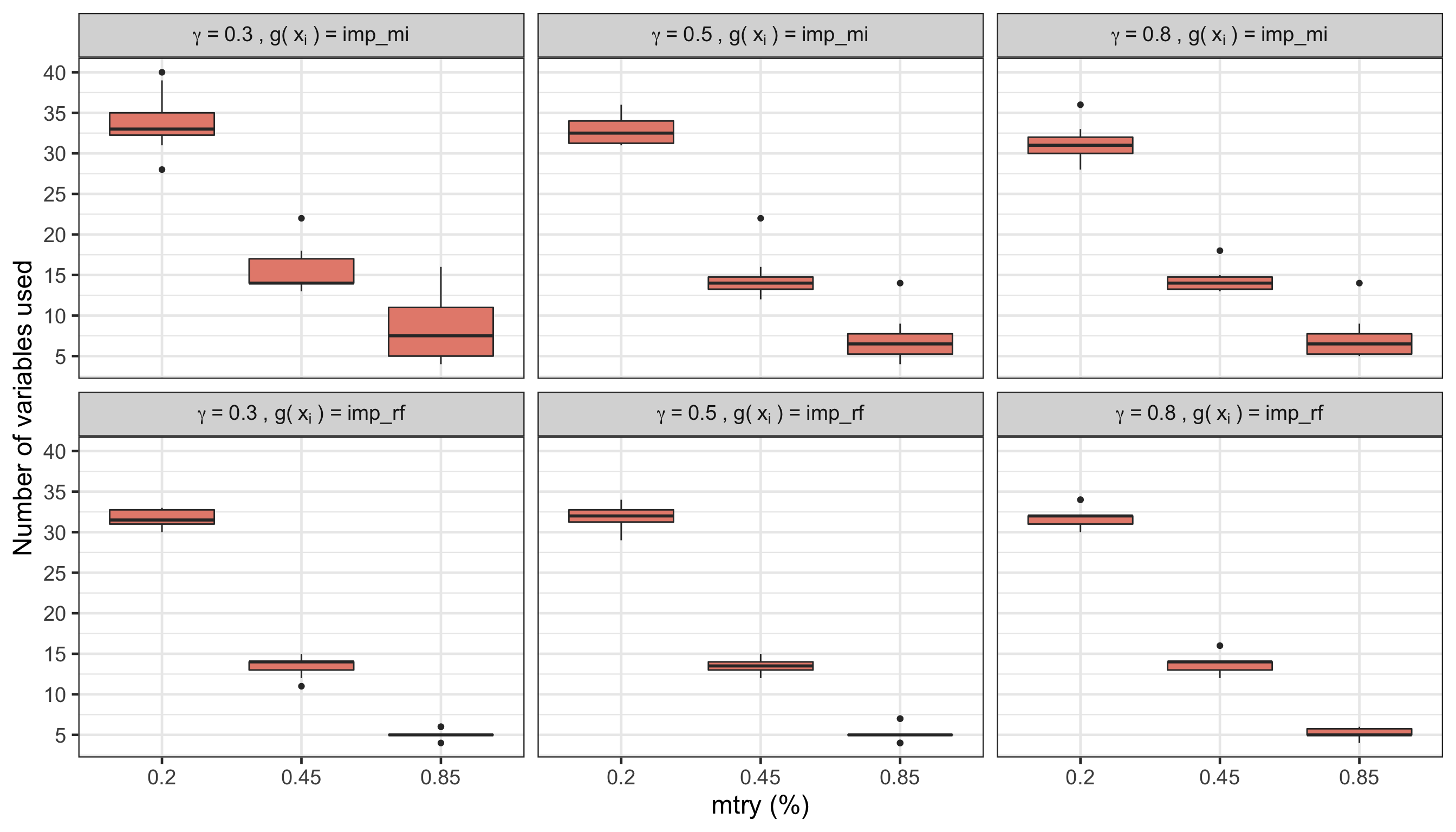
Figure 2: Figure 2. Final number of variables used for each combination of mtry, type of $g(\mathbf{x}_i)$, and $\gamma$

From the plots above, we can have an idea of what the test accuracies (Figure 1) and final number of variables used (Figure 2) is for each combination of mtry (in percentage of variables used), and type of $g(\mathbf{x}_i)$ (using a mutual information function or boosted by a standard RF), marginalized over $\lambda_0$. Comparing that to the test accuracy (average of 0.744) and number of variables used (average of 1308) of the standard random forest, we can see that there has been a good improvement, since most models have a simelar accuracy to a full random forest, but are using many fewer features (from a maximum of around 30 to a minimum of around 5 features). Regarding the hyperparameter configurations, it seems that using the normalized importance values of a standard random forest as $g(\mathbf{x}_i)$ leads to the best test accuracy results overall, but with more variation across the different mtry values. As for the number of features used, using the normalized importance values of a standard random forest as $g(\mathbf{x}_i)$ results in using just a few variables, also with a bigger variation across mtry values. The number of features used for this scenario gets very low, which can be very attractive if we’re worried about using the least variables as possible.

Now, following what was described before as the ‘full feature selection procedure’, let’s move on to the next step: selecting the best penalized models for each training set and reevaluating them. In the next code chunks, we get the top-3 models for each training id, arranging first by test accuracy, training accuracy and number of variables. After that, we create the new model formulas for each model, rerun the random forest algorithm with each feature set, for each of the 5 training sets and evaluate their results:


best_models <- results %>% 
  arrange(desc(accuracy_test), desc(accuracy), n_var) %>% 
  group_by(id) %>% 
  slice(1:3) %>% 
  ungroup() %>% 
  mutate(new_formula = map(model_importance, get_formula))

# Re-evaluating selected variables -----------------
reev <- tibble(forms = best_models$new_formula) %>% 
  tidyr::expand_grid(folds) %>% 
  dplyr::mutate(reev_models = purrr::map2(train, forms, modelling_reev))

results_reev <- reev %>% 
  dplyr::mutate(feat_importance = purrr::map(reev_models, ~{.x$fit$variable.importance}),
                n_var = purrr::map_dbl(feat_importance, n_vars),
                accuracy = 1 - purrr::map_dbl(reev_models, ~{ .x$fit$prediction.error}),
                accuracy_test = purrr::map2_dbl(.x = reev_models, .y = test, ~{ acc_test(.x, test = .y)}))

id	n_var	accuracy	accuracy_test
Fold2	31	0.8638687	0.971
Fold2	31	0.8768484	0.941
Fold2	12	0.8650016	0.941
Fold3	5	0.8607979	0.941
Fold2	5	0.8566280	0.941

The accuracy values are looking very good now, even for the test set. Note that the results_reev object has 75 rows, since we have run 15 random forests models for each of the 5 training sets. We still need to reduce this number, so the last step of our methods consists of gathering the most used features by such models, and creating one final algorithm. This final model will be evaluated in 20 training and test sets, so we can be more certain about its accuracy results. In the following code, we select the top best 30 fitted models (in terms of the accuracies and number of features used) find the 15 features most used by them, and fit a random forest model in the 20 new training and test sets using this final 15-features set.


selected_vars <- results_reev %>% 
  arrange(desc(accuracy_test), desc(accuracy), n_var) %>% 
  slice(1:30) %>% 
  mutate(ind = 1:n(), vars = map(feat_importance, get_vars)) %>% 
  dplyr::select(ind, vars) %>% 
  unnest() %>% 
  group_by(vars) %>% 
  summarise(count = n()) %>% 
  arrange(desc(count))

# Select the final 15 features
final_vars <- selected_vars %>% slice(1:15) %>% pull(vars)
# Create the final formula 
final_form <- paste("class ~ ", paste0(final_vars, collapse = ' + ')) %>%
  as.formula()

# Create the 20 new training and test sets
set.seed(2021)
folds_20 <- rsample::vfold_cv(gravier, v = 20) %>% 
  dplyr::mutate(train =  map(splits, training), test  = map(splits, testing))

# Run the final model for the new train-test sets
final_results <- folds_20$splits %>% map(~{
  train <-  training(.x)
  test <-  testing(.x)
  
  rf <- rand_forest(trees = 500, mtry = 7) %>%
    set_engine("ranger", importance = "impurity") %>% 
    set_mode("classification") %>% 
    parsnip::fit(final_form, data = train)
  
  accuracy_test <- acc_test(rf, test = test)
  list(accuracy_test = accuracy_test, 
       accuracy = 1 - rf$fit$prediction.error, 
       imp = rf$fit$variable.importance)
})

The accuracy averages and medians for this final model are shown below. We can see that the final test accuracy (average) is higher than what was seen in the previous plots, but now using only 15 features. At last, we show the variable importance plot for the 15 features used, arranged by importance order. This plot informs us about which variables helped the predictions the most, and we can see that the most important feature really dominates the plot.


data.frame(accuracy_test = final_results %>% map_dbl("accuracy_test"), 
           accuracy = final_results %>% map_dbl("accuracy")) %>% 
  gather(type, value) %>% 
  group_by(type) %>% 
  summarise(mean = mean(value), median = median(value))

type	mean	median
accuracy	0.8974934	0.8971951
accuracy_test	0.8681000	0.8820000

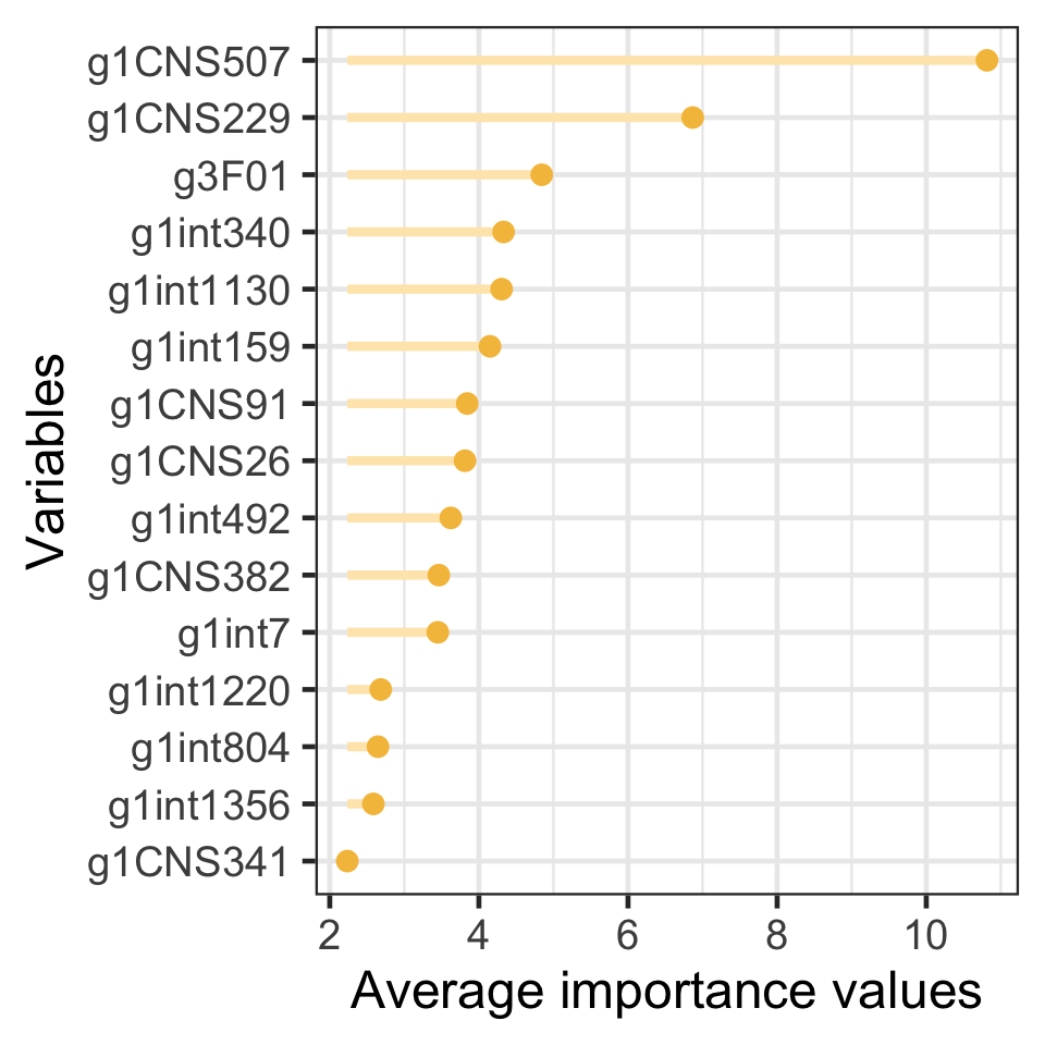
Figure 3: Figure 3. Average importance values for the final selected variables

How does this compare to the literature?

This post only intends to quickly demonstrate how the feature selection via gain penalization can be used, but we can also compare our results to a few others that have come up in similar literature that used the same dataset:

(Huynh, Do, and others 2020) reports a maximum accuracy of 84.52% (page 10)
(López, Maldonado, and Carrasco 2018) reports a maximum AUC of 79.7 (page 384)
(Takada, Suzuki, and Fujisawa 2018) reports a maximum miscalssification accuracy of ~75% (page 9)

Breiman, Leo. 1996. “Bagging Predictors.” Machine Learning 24 (2): 123–40. https://doi.org/10.1023/A:1018054314350.

Deng, Houtao, and George Runger. 2012. “Feature Selection via Regularized Trees.” In The 2012 International Joint Conference on Neural Networks (Ijcnn), 1–8. IEEE.

Gravier, Eléonore, Gaëlle Pierron, Anne Vincent-Salomon, Nadège Gruel, Virginie Raynal, Alexia Savignoni, Yann De Rycke, et al. 2010. “A Prognostic Dna Signature for T1t2 Node-Negative Breast Cancer Patients.” Genes, Chromosomes and Cancer 49 (12): 1125–34.

Huynh, Phuoc-Hai, Thanh-Nghi Do, and others. 2020. “Improvements in the Large P, Small N Classification Issue.” SN Computer Science 1 (4): 1–19.

Louppe, Gilles. 2014. “Understanding Random Forests: From Theory to Practice.” PhD thesis. https://doi.org/10.13140/2.1.1570.5928.

López, Julio, Sebastián Maldonado, and Miguel Carrasco. 2018. “Double Regularization Methods for Robust Feature Selection and Svm Classification via Dc Programming.” Information Sciences 429: 377–89.

Takada, Masaaki, Taiji Suzuki, and Hironori Fujisawa. 2018. “Independently Interpretable Lasso: A New Regularizer for Sparse Regression with Uncorrelated Variables.” In International Conference on Artificial Intelligence and Statistics, 454–63. PMLR.

Wundervald, Bruna, Andrew C Parnell, and Katarina Domijan. 2020. “Generalizing Gain Penalization for Feature Selection in Tree-Based Models.” IEEE Access 8: 190231–9.

Feature Selection via Gain Penalization in Random Forests

Table of Contents